Please click on their logo below to visit their website and see the many free and paid-for Google Sheets solutions in their portfolio.

Your typical Excel user is probably a little prejudiced when it comes to Google Sheets:
“Isn’t it the same but slightly worse imitation of Microsoft Excel?” The reality is that this is far from the truth, and this article will explore some of the novelties Google Sheets has brought to the world of spreadsheets.
There are obvious benefits (which are the common features across the Google products workspace) such as simultaneous multi-user editing and easy online sharing which made Google a pioneer in the era of online collaboration. However, Google Sheets can be very proud of the improvements and alternative approaches it has brought to the spreadsheet space in recent years which address the habitual problems which users face.
So let’s explore 10 unique features of Google Sheets together!
One of the great features of Google Sheets is the way you can use array functions. Arrays are not new to spreadsheet programs, especially not in Excel. However, Google Sheets allows its user to use arrays from a new perspective that is less complex and user-friendly.
One thing you can do with array functions in Google Sheets is to use it to organize separated pieces of data on the spreadsheet. Think it like that: Your customer sent you a spreadsheet where the income range starts in A3 (why is never a related question in the industry) whereas the income sources are stated in a different place. You can organize these ranges beside each other with an array formula.
All you need to do is open an array and state the data you want to be put according to each other by commas and semicolons such as below:
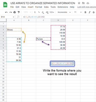
={A3,C6;A6:A13,D2:D9}
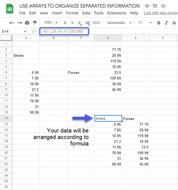
Commas separate the columns and semicolons separate the rows.
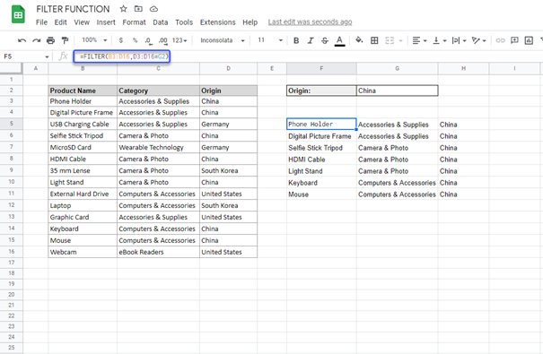
Another function in Google Sheets that would make your job easier is the filter function. It takes a range of data, and it takes a condition to filter it. With this feature, you can handle filtering will be easy and it can be integrated into formulas.
Example:
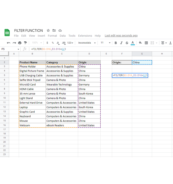
=FILTER(B4:D17,D4:D17=F5)
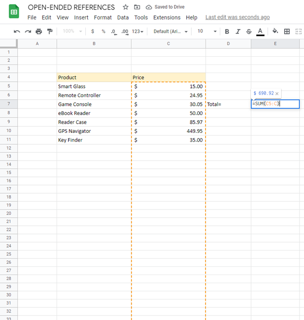
If you are going to add more data to your balance sheet in the future, open references will be a great help for the total calculations. Because you can do open-ended cell references in Google Sheets, you can write an open-ended SUM formula. That way, when you write new numbers in the column, the sum will change automatically.
Import features in Google Sheets are in fact exciting! You can import a table or a list from a web page to your Google Sheets file with the IMPORTHTML function. Let’s say you want to integrate the List of countries by nominal GDP from Wikipedia into your spreadsheet. Google Sheets provides you with the easiest way for it! With the formula below, you can pull data from the web!
=IMPORTHTML(“url”, “query”, index, locale)
=IMPORTHTML(“https://en.wikipedia.org/wiki/List_of_countries_by_GDP_(nominal)”, “Table”, 4)
The formula above will give you what you want from the web page.

Query function is highly helpful to those who use spreadsheets for their work (or in daily life) because you can use it instead of many other formulas such as Filter, Sort, Unique, etc. Because it is versatile and multi-dimensional, we can’t really show you all the things you can do with Query.
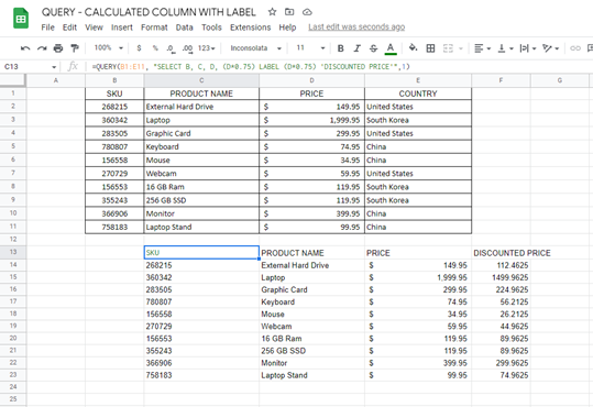
Instead, we’re going to show you one very useful trick with the Query function. If you have a table of data and you want to create an additional column where you can calculate values in the table, Query function provides an easy way.
Let’s say that you have the table of data below:

Let’s assume that you will have a sale of 25% for these products. You can calculate the discounted price and show them in a separate column with the query function. You can write the formula below and the table below will automatically appear.
=QUERY(B1:E11, “SELECT B, C, D, (D*0.75) LABEL (D*0.75) ‘DISCOUNTED PRICE'”,1)

Sparklines are basically small simple charts that sit in the cells! They provide a visual representation of data within a single cell in a spreadsheet. Sparklines in Google Sheets are used to show trends or patterns in data, without taking up much space.
To create a sparkline in Google Sheets, you can use the following steps:
Select the cell where you want the sparkline to appear and type the sparkline formula. To create a sparkline you need to determine two things in the formula. The data and the type of sparkline you want to create (e.g. Line, Column, or Win/Loss).
Let me show you how you can use sparkline to create different charts:
To create a sparkline from a column, you need to determine the data range and the other features (options) in the SPARKLINE formula as below:
=SPARKLINE(datarange,{options})
As you can see you can write color as an option.
You can also determine the chart type, the linewidth of the chart columns/lines, or max and min values in the chart. Let us show another sparkline to you as a bar chart:

The option in the example above includes color, linewidth, ymax and min values, and chart type as options. So, the formula is:
=SPARKLINE(D4:D15,{“color”,”purple”;”linewidth”,3;”ymin”,300;”ymax”,3000;”charttype”,”column”})
Because Google Sheets is a Google product, you can use other Google technologies within your Google Sheets files easily. Detect Language is one of them. If you have a column or a row in a different language and you want to detect the content’s language or translate the content, what you can do to is to write the simple formula below:
=DETECTLANGUAGE(text_or_range)

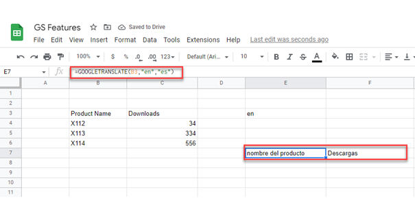
Similarly, you can also translate the text in a cell with the GOOGLE TRANSLATE function. The important point here is that the formula for Google Translate doesn’t support ranges. To translate an entire row, you can use the formula for one cell and then copy paste it to apply to the other cells in the column or row.
You should use the formula below to translate a cell or text from one language to other:
=GOOGLETRANSLATE(text,”source_language”,”target_language”)
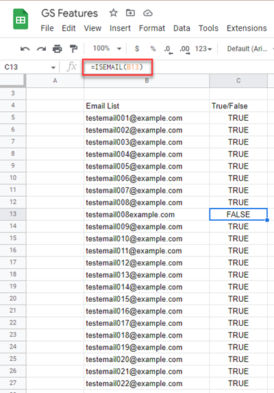
Let’s say you have hundreds of email addresses that you will use in a campaign. However, the data file includes names or URLs as well as email addresses. How will you collect the email addresses easily? Well, Google Sheets offers the simplest function for that. All you need to write is the formula below and it will tell you if the cell contains an email address or not.
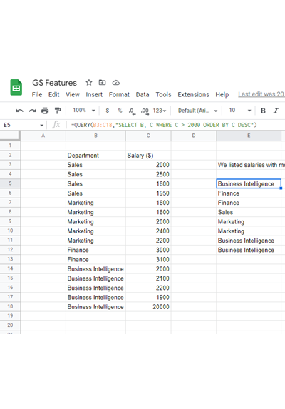
Query is a great function if you need to process data with different functions at the same time. For example, if you want to filter data and also want to sort it in a specific way simultaneously, Query offers you an easy solution. In the example below, we have different salaries from different departments. Let’s say you want to list salaries with more than $2000 but you must have them sorted from greatest to smallest amount. You can just use a Query function:
QUERY(A2:E6, “select avg(A) pivot B”, -1)
Another solution query offers are to provide the total sum of your data while also categorizing them according to your needs. To clarify, let’s assume an example:
You have a list of various products and their order amounts per day randomly. You want to see the total orders per product category. The easiest way to filter this information is by implementing a query in Google Sheets.
By writing a similar formula below, you can ask for the results of the sum of a range within related groups.
=QUERY(B2:C31,”SELECT range, sum(range) GROUP BY range”)
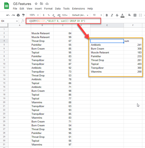
As you can see, the query grouped product categories and showed the sum of them in the next column.
Conclusion:
Google Sheets definitely make teamwork easier and provide new solutions for its users way never previously imagined. If you are not a developer and have a requirement which necessitates a bespoke solution please feel free to reach out to our team of Expert Developers at FD4Cast and/or Someka.net.